pacman::p_load(ggstatsplot, tidyverse)Hands-on Exercise 4a
Getting Started
Install and launching R packages
The code chunk below uses p_load() of pacman package to check if ggstatsplot and tidyverse packages are installed in the computer. If they are, then they will be launched into R.
Importing the data
exam_data <- read_csv("data/Exam_data.csv", show_col_types = FALSE)Statistical Tests
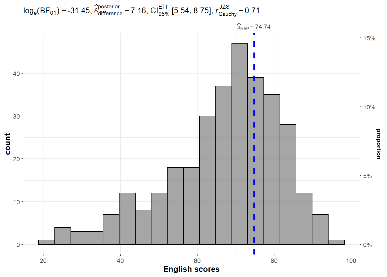
One-sample Test: gghistostats()
Code
set.seed(1234)

gghistostats(
  data = exam_data,
  x = ENGLISH,
  type = "bayes",
  test.value = 60,
  xlab = "English scores"
)
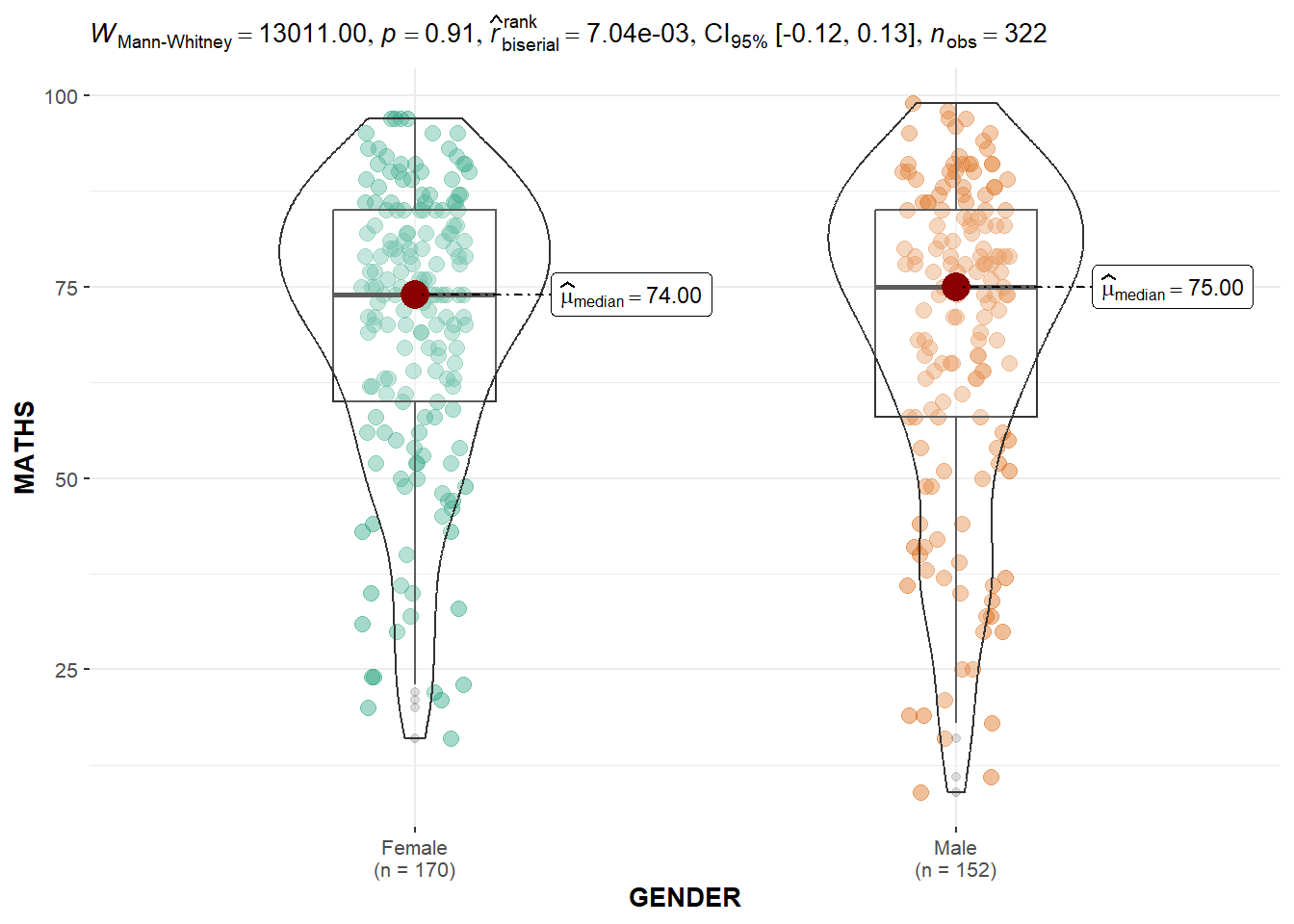
Two-sample Mean Test: ggbetweenstats()
Code
ggbetweenstats(
  data = exam_data,
  x = GENDER,
  y = MATHS,
  type = "np",
  messages = FALSE
)
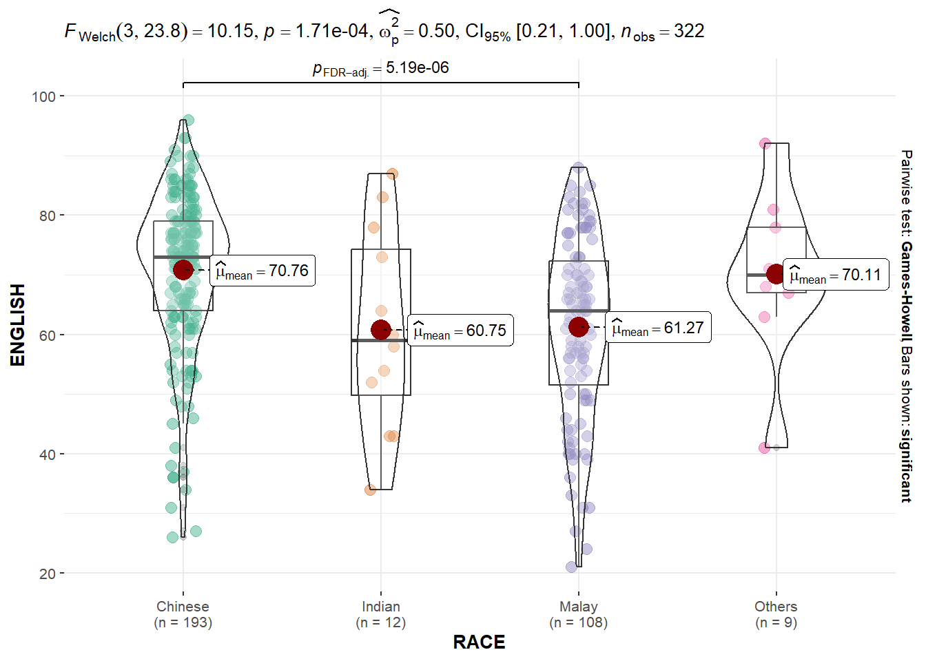
Oneway ANOVA Test: ggbetweenstats()
Code
ggbetweenstats(
  data = exam_data,
  x = RACE,
  y = ENGLISH,
  type = "p",
  mean.ci = TRUE,
  pairwise.comparisons = TRUE,
  pairwise.display = "s",
  p.adjust.method = "fdr",
  messages = FALSE
)
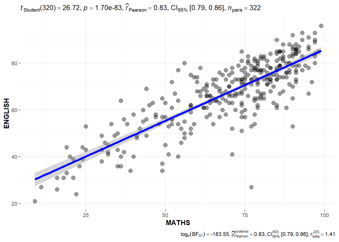
Significant Test of Correlation: ggscatterstats()
Code
ggscatterstats(
  data = exam_data,
  x = MATHS,
  y = ENGLISH,
  marginal = FALSE,
  )
Significant Test of Association (Depedence): ggbarstats()
For this section, the Math scores are binned into 4 classes using cut().
exam1 <- exam_data %>%
  mutate(MATHS_bins =
           cut(MATHS,
               breaks = c(0,60,75,85,100))
)
Code
ggbarstats(exam1,
           x = MATHS_bins,
           y = GENDER)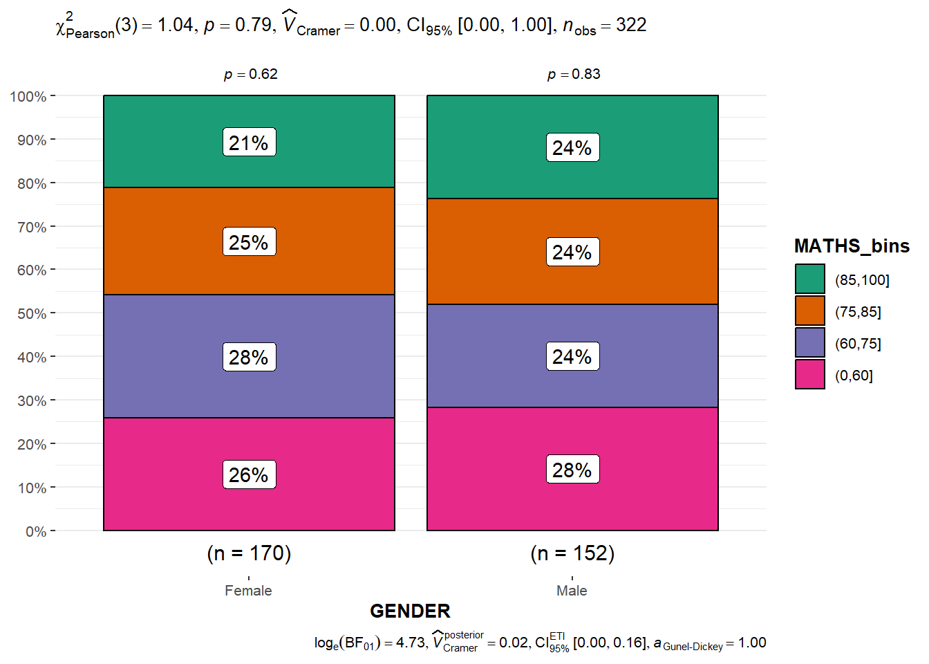
Visualising Models
realxl() is used to import the data worksheet of ToyotaCorolla.xls workbook into R.
pacman::p_load(readxl, performance, parameters, see)car_resale <- read_xls("data/ToyotaCorolla.xls",
"data")
car_resale# A tibble: 1,436 × 38
Id Model Price Age_08_04 Mfg_Month Mfg_Year KM Quarterly_Tax Weight
<dbl> <chr> <dbl> <dbl> <dbl> <dbl> <dbl> <dbl> <dbl>
1 81 TOYOTA … 18950 25 8 2002 20019 100 1180
2 1 TOYOTA … 13500 23 10 2002 46986 210 1165
3 2 TOYOTA … 13750 23 10 2002 72937 210 1165
4 3 TOYOTA… 13950 24 9 2002 41711 210 1165
5 4 TOYOTA … 14950 26 7 2002 48000 210 1165
6 5 TOYOTA … 13750 30 3 2002 38500 210 1170
7 6 TOYOTA … 12950 32 1 2002 61000 210 1170
8 7 TOYOTA… 16900 27 6 2002 94612 210 1245
9 8 TOYOTA … 18600 30 3 2002 75889 210 1245
10 44 TOYOTA … 16950 27 6 2002 110404 234 1255
# ℹ 1,426 more rows
# ℹ 29 more variables: Guarantee_Period <dbl>, HP_Bin <chr>, CC_bin <chr>,
# Doors <dbl>, Gears <dbl>, Cylinders <dbl>, Fuel_Type <chr>, Color <chr>,
# Met_Color <dbl>, Automatic <dbl>, Mfr_Guarantee <dbl>,
# BOVAG_Guarantee <dbl>, ABS <dbl>, Airbag_1 <dbl>, Airbag_2 <dbl>,
# Airco <dbl>, Automatic_airco <dbl>, Boardcomputer <dbl>, CD_Player <dbl>,
# Central_Lock <dbl>, Powered_Windows <dbl>, Power_Steering <dbl>, …Multiple Regression Model using lm()
model <- lm(Price ~ Age_08_04 + Mfg_Year + KM +
              Weight + Guarantee_Period, data = car_resale)
model
Call:
lm(formula = Price ~ Age_08_04 + Mfg_Year + KM + Weight + Guarantee_Period,
    data = car_resale)

Coefficients:
     (Intercept)         Age_08_04          Mfg_Year                KM
      -2.637e+06        -1.409e+01         1.315e+03        -2.323e-02
          Weight  Guarantee_Period
       1.903e+01         2.770e+01
Checking for Collinearity
check_collinearity(model)# Check for Multicollinearity
Low Correlation
Term VIF VIF 95% CI Increased SE Tolerance Tolerance 95% CI
KM 1.46 [ 1.37, 1.57] 1.21 0.68 [0.64, 0.73]
Weight 1.41 [ 1.32, 1.51] 1.19 0.71 [0.66, 0.76]
Guarantee_Period 1.04 [ 1.01, 1.17] 1.02 0.97 [0.86, 0.99]
High Correlation
Term VIF VIF 95% CI Increased SE Tolerance Tolerance 95% CI
Age_08_04 31.07 [28.08, 34.38] 5.57 0.03 [0.03, 0.04]
Mfg_Year 31.16 [28.16, 34.48] 5.58 0.03 [0.03, 0.04]check_c <- check_collinearity(model)
plot(check_c)Variable `Component` is not in your data frame :/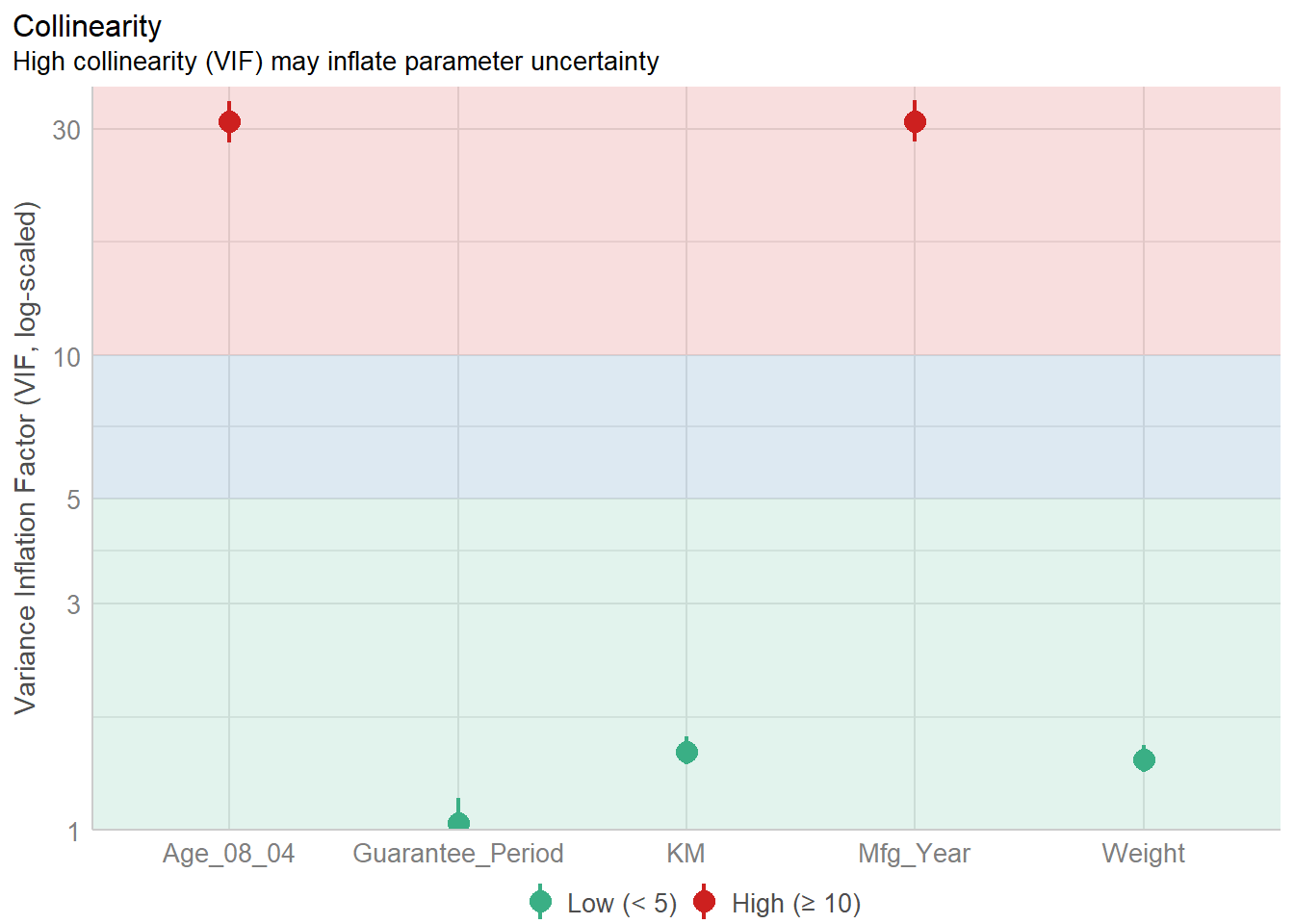
Checking for Normality Assumption
model1 <- lm(Price ~ Age_08_04 + KM +
              Weight + Guarantee_Period, data = car_resale)
check_n <- check_normality(model1)plot(check_n)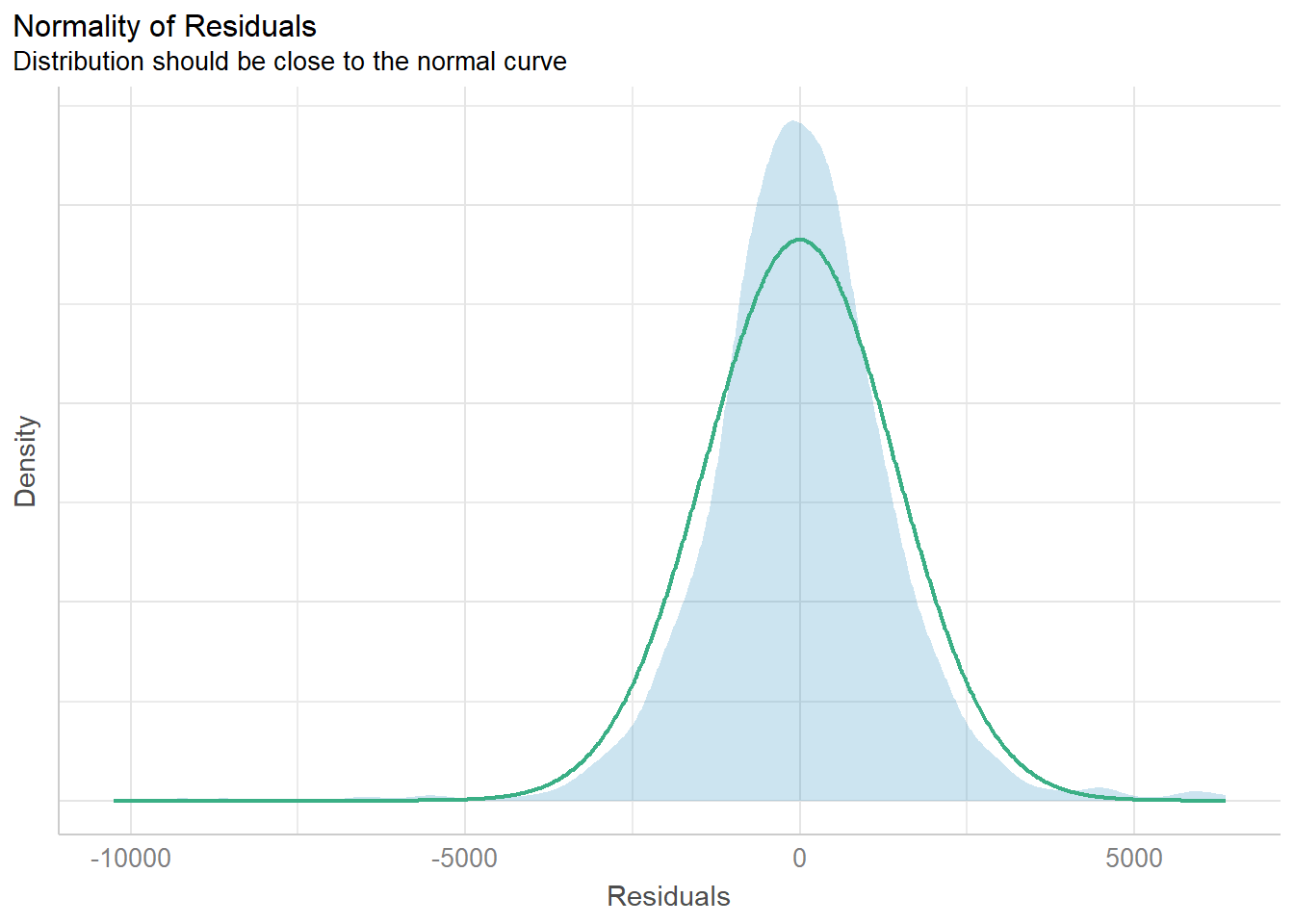
Checking for Homogeneity of Variances
check_h <- check_heteroscedasticity(model1)plot(check_h)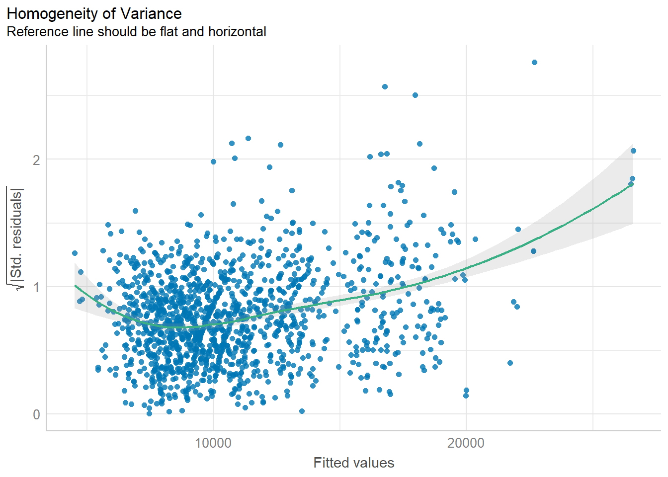
Alternative: Complete Check
check_model(model1)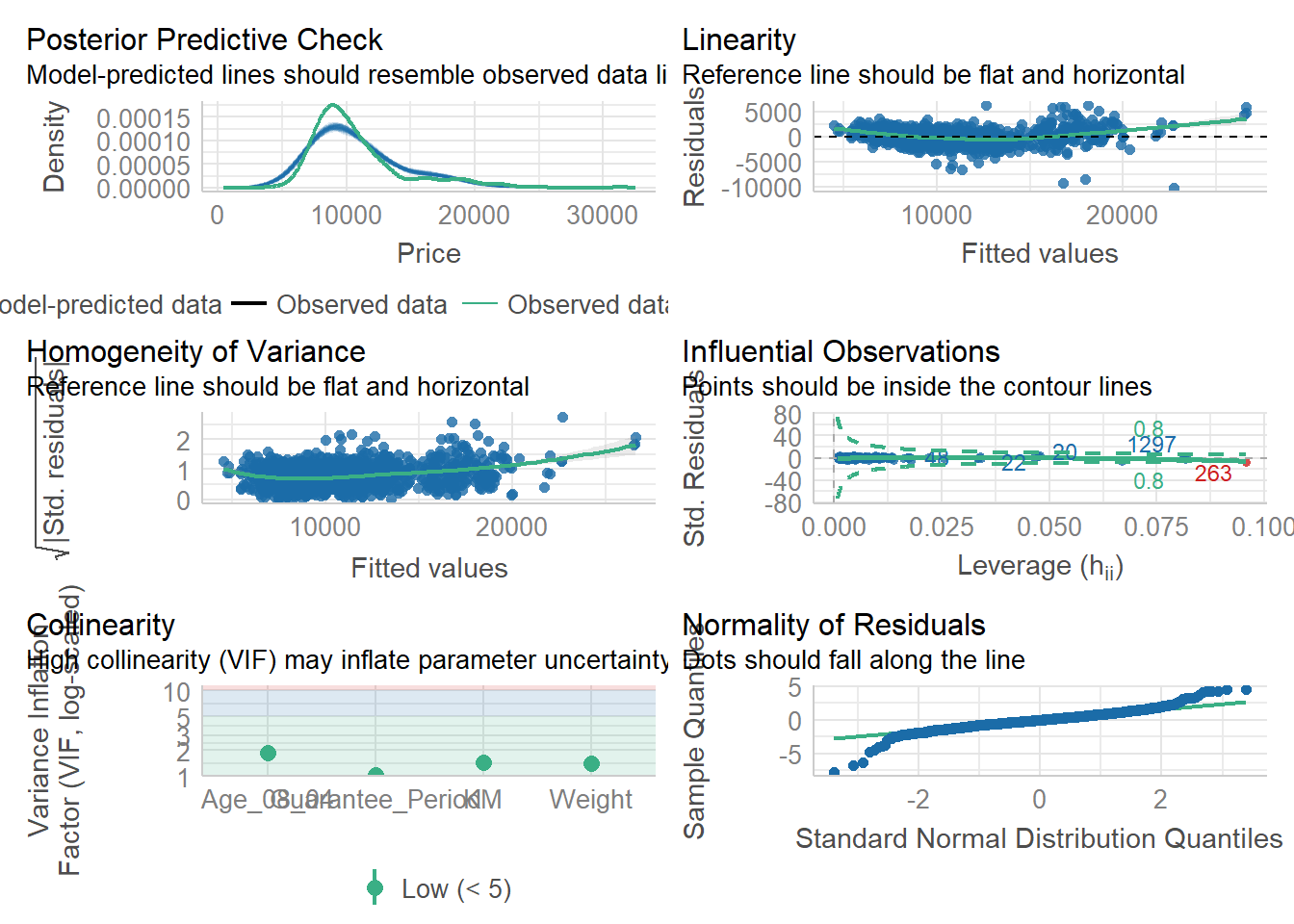
Visualizing Regression Parameters
Method 1
plot(parameters(model1))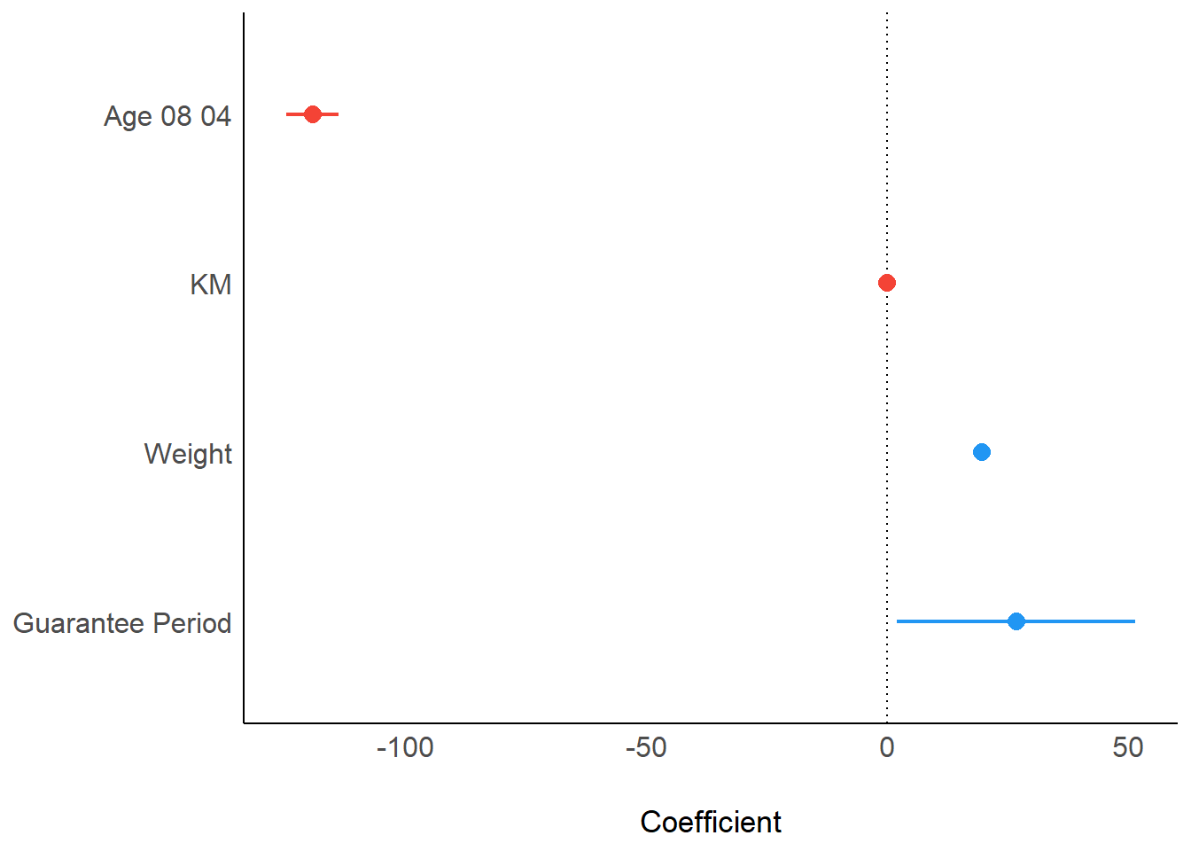
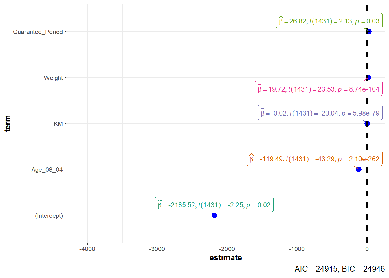
Method 2
ggcoefstats(model1,
            output = "plot")