pacman::p_load(igraph, tidygraph, ggraph,
               visNetwork, lubridate, clock,
tidyverse, graphlayouts)In-class Exercise 5
Getting Started
Install and launching R packages
The code chunk below uses p_load() of pacman package to check if the relevant packages are installed in the computer. If they are, then they will be launched into R.
Importing the data
GAStech_nodes <- read_csv("data/GAStech_email_node.csv")
GAStech_edges <- read_csv("data/GAStech_email_edge-v2.csv")
Wrangling time data
GAStech_edges <- GAStech_edges %>%
  mutate(SendDate = dmy(SentDate)) %>%
  mutate(Weekday = wday(SentDate,
                        label = TRUE,
                        abbr = FALSE))
Wrangling other attributes
GAStech_edges_aggregated <- GAStech_edges %>%
  filter(MainSubject == "Work related") %>%
  group_by(source, target, Weekday) %>%
    summarise(Weight = n()) %>%
  filter(source!=target) %>%
  filter(Weight > 1) %>%
  ungroup()
Creating network objects using tidygraph
GAStech_graph <- tbl_graph(nodes = GAStech_nodes,
                           edges = GAStech_edges_aggregated,
                           directed = TRUE)
Changing the active object
GAStech_graph %>%
  activate(edges) %>%
  arrange(desc(Weight))
# A tbl_graph: 54 nodes and 1372 edges
#
# A directed multigraph with 1 component
#
# A tibble: 1,372 × 4
from to Weekday Weight
<int> <int> <ord> <int>
1 40 41 Saturday 13
2 41 43 Monday 11
3 35 31 Tuesday 10
4 40 41 Monday 10
5 40 43 Monday 10
6 36 32 Sunday 9
# ℹ 1,366 more rows
#
# A tibble: 54 × 4
id label Department Title
<dbl> <chr> <chr> <chr>
1 1 Mat.Bramar Administration Assistant to CEO
2 2 Anda.Ribera Administration Assistant to CFO
3 3 Rachel.Pantanal Administration Assistant to CIO
# ℹ 51 more rowsPlotting network graphs with ggraph
Plotting a basic graph
ggraph(GAStech_graph) +
  geom_edge_link() +
  geom_node_point()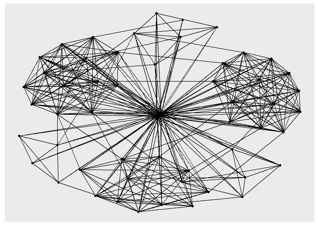
Changing the theme
g <- ggraph(GAStech_graph) +
  geom_edge_link(aes()) +
  geom_node_point(aes())

g + theme_graph()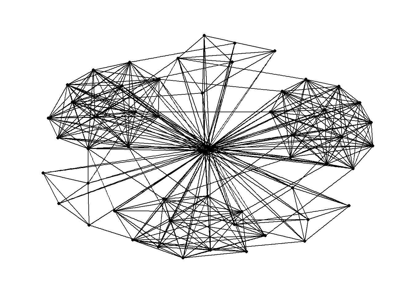
Changing the plot colour
g <- ggraph(GAStech_graph) +
  geom_edge_link(aes(colour = 'grey50')) +
  geom_node_point(aes(colour = 'grey40'))

g + theme_graph(background = 'grey10',
                text_colour = 'white')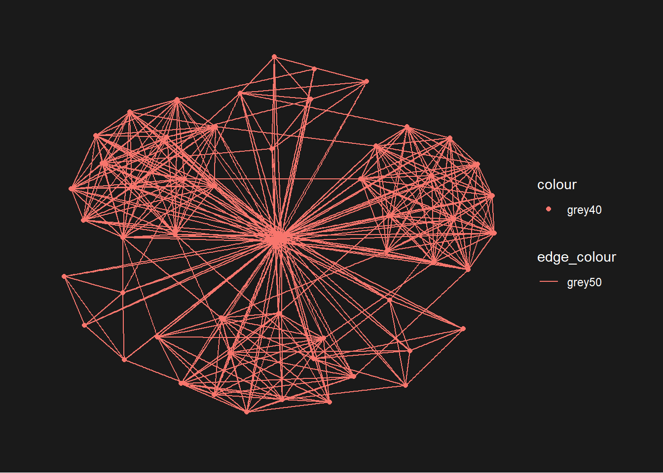
Working with ggraph layouts
g <- ggraph(GAStech_graph,
            layout = "fr") +
  geom_edge_link(aes()) +
  geom_node_point(aes()) +
  ggtitle("Fruchterman and Reingold layout")

g + theme_graph()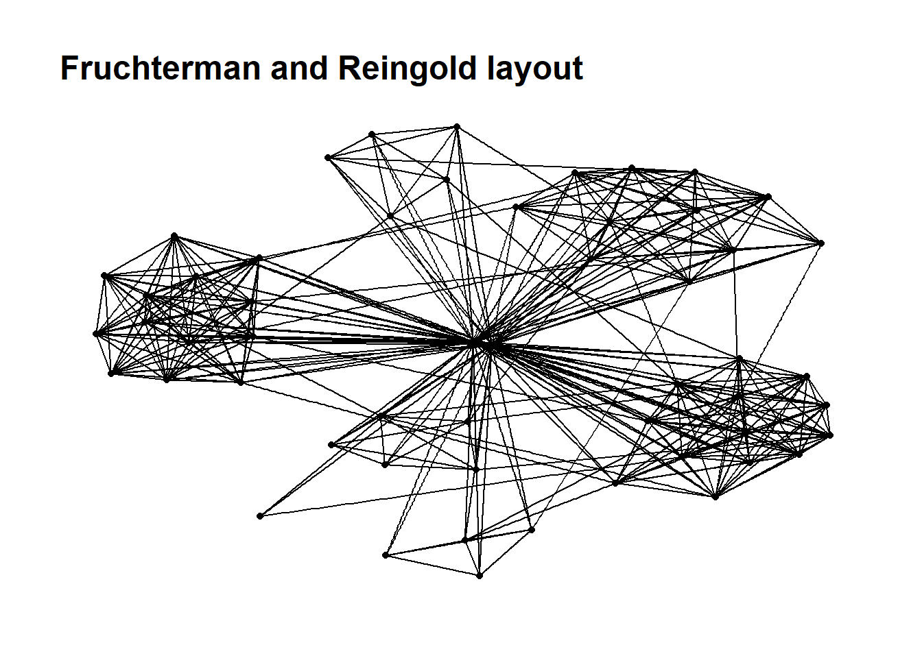
Modifying network nodes
g <- ggraph(GAStech_graph,
            layout = "nicely") +
  geom_edge_link(aes()) +
  geom_node_point(aes(colour = Department,
                      size = 3))

g + theme_graph()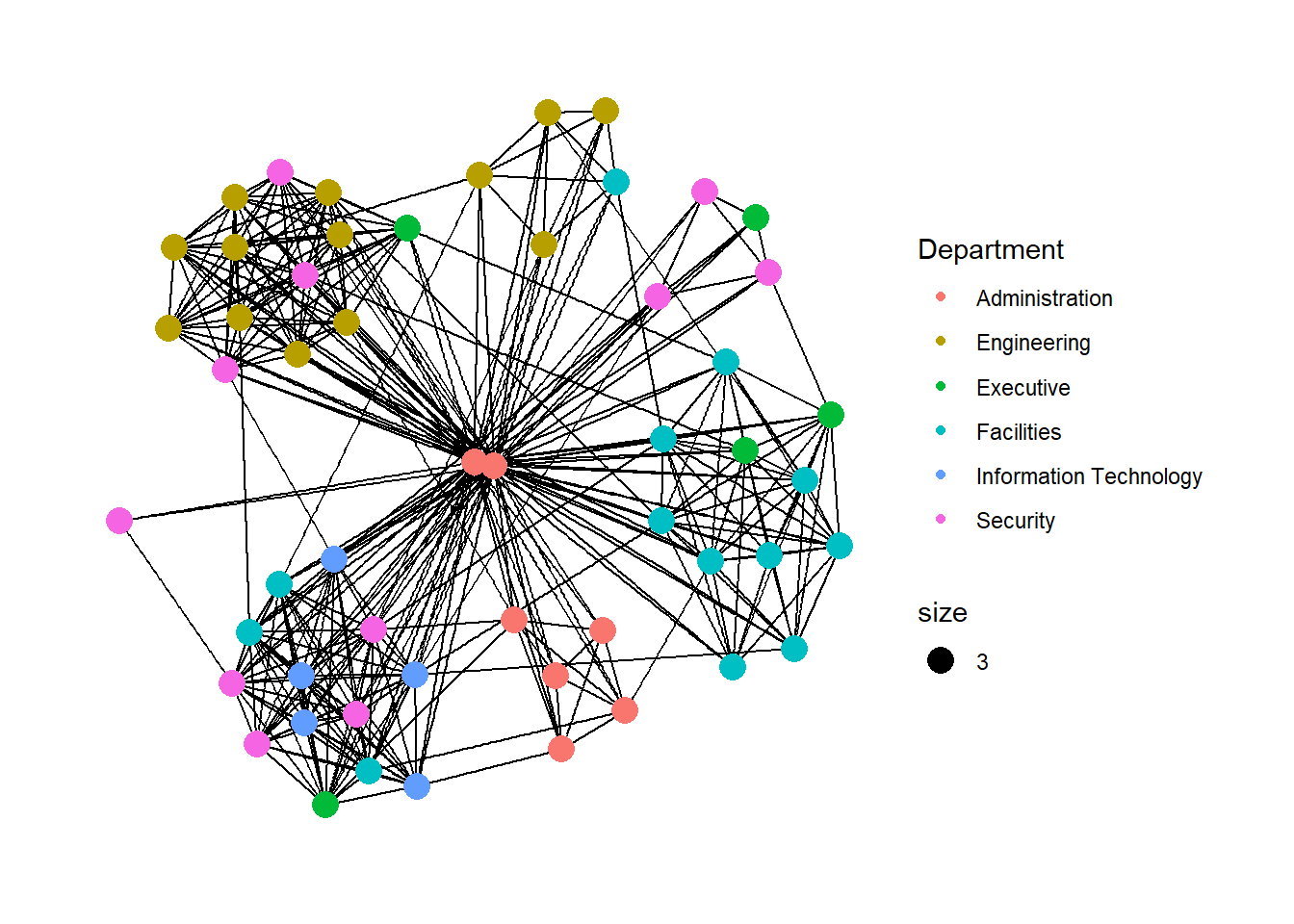
Modifying edges
g <- ggraph(GAStech_graph,
            layout = "nicely") +
  geom_edge_link(aes(width=Weight),
                 alpha=0.2) +
  scale_edge_width(range = c(0.1, 5)) +
  geom_node_point(aes(colour = Department),
                  size = 3)

g + theme_graph()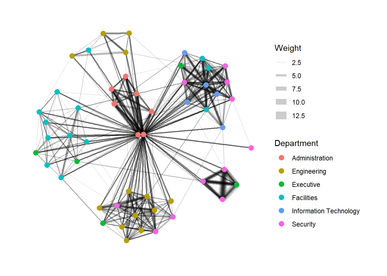
Creating facet graphs
Working with facet_edges()
set_graph_style()

g <- ggraph(GAStech_graph,
            layout = "nicely") +
  geom_edge_link(aes(width=Weight),
                 alpha=0.2) +
  scale_edge_width(range = c(0.1, 5)) +
  geom_node_point(aes(colour = Department),
                  size = 2)

g + facet_edges(~Weekday)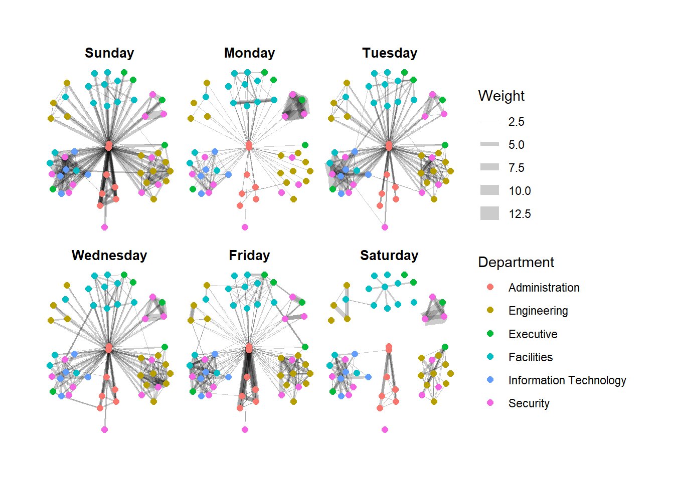
set_graph_style()

g <- ggraph(GAStech_graph,
            layout = "nicely") +
  geom_edge_link(aes(width=Weight),
                 alpha=0.2) +
  scale_edge_width(range = c(0.1, 5)) +
  geom_node_point(aes(colour = Department),
                  size = 2) +
  theme(legend.position = 'bottom')

g + facet_edges(~Weekday)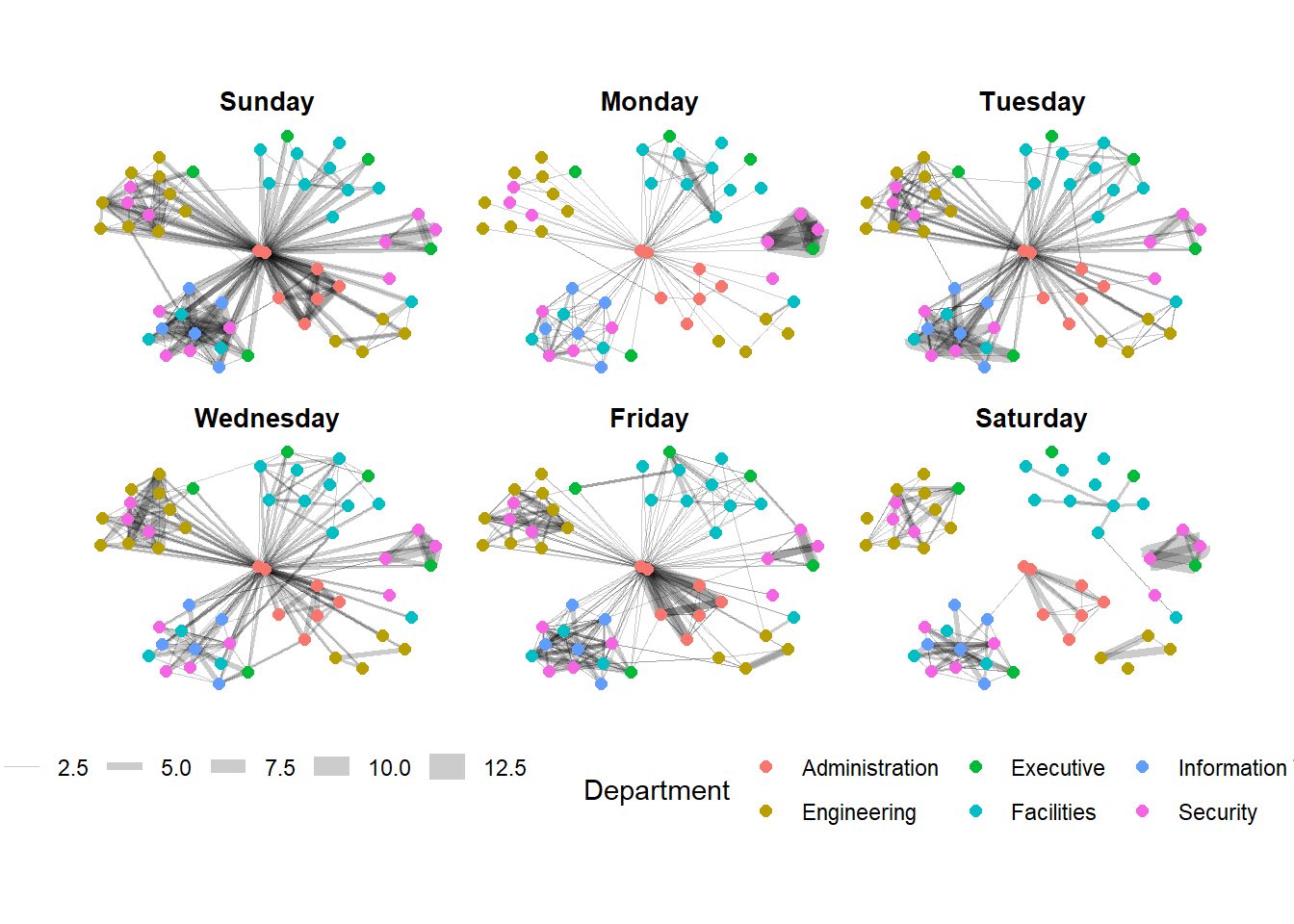
Framed facet graph
set_graph_style()

g <- ggraph(GAStech_graph,
            layout = "nicely") +
  geom_edge_link(aes(width=Weight),
                 alpha=0.2) +
  scale_edge_width(range = c(0.1, 5)) +
  geom_node_point(aes(colour = Department),
                  size = 2)

g + facet_edges(~Weekday) +
  th_foreground(foreground = "grey80",
                border = TRUE) +
  theme(legend.position = 'bottom')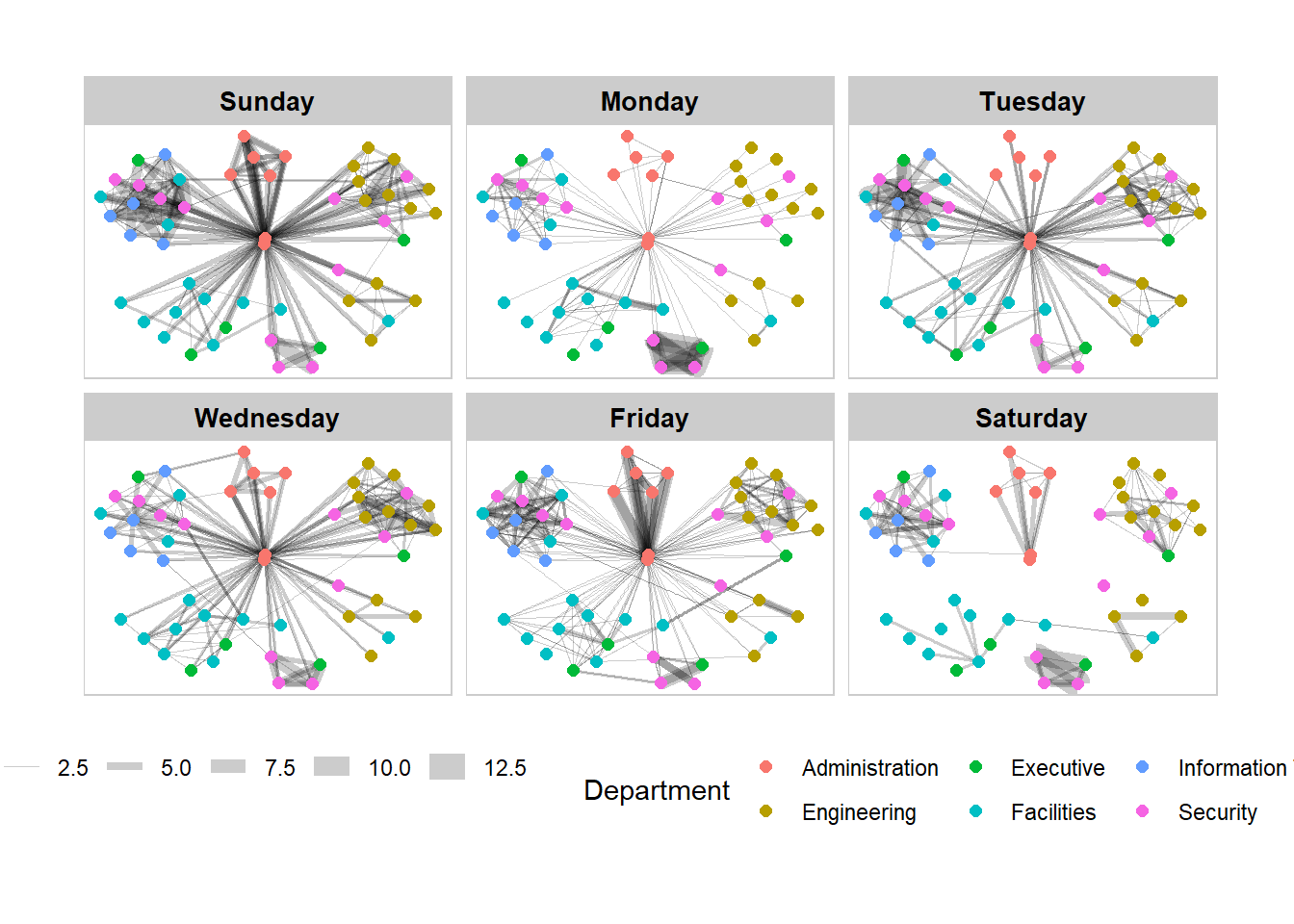
Working with facet_nodes()
set_graph_style()

g <- ggraph(GAStech_graph,
            layout = "nicely") +
  geom_edge_link(aes(width=Weight),
                 alpha=0.2) +
  scale_edge_width(range = c(0.1, 5)) +
  geom_node_point(aes(colour = Department),
                  size = 2)

g + facet_nodes(~Department)+
  th_foreground(foreground = "grey80",
                border = TRUE) +
  theme(legend.position = 'bottom')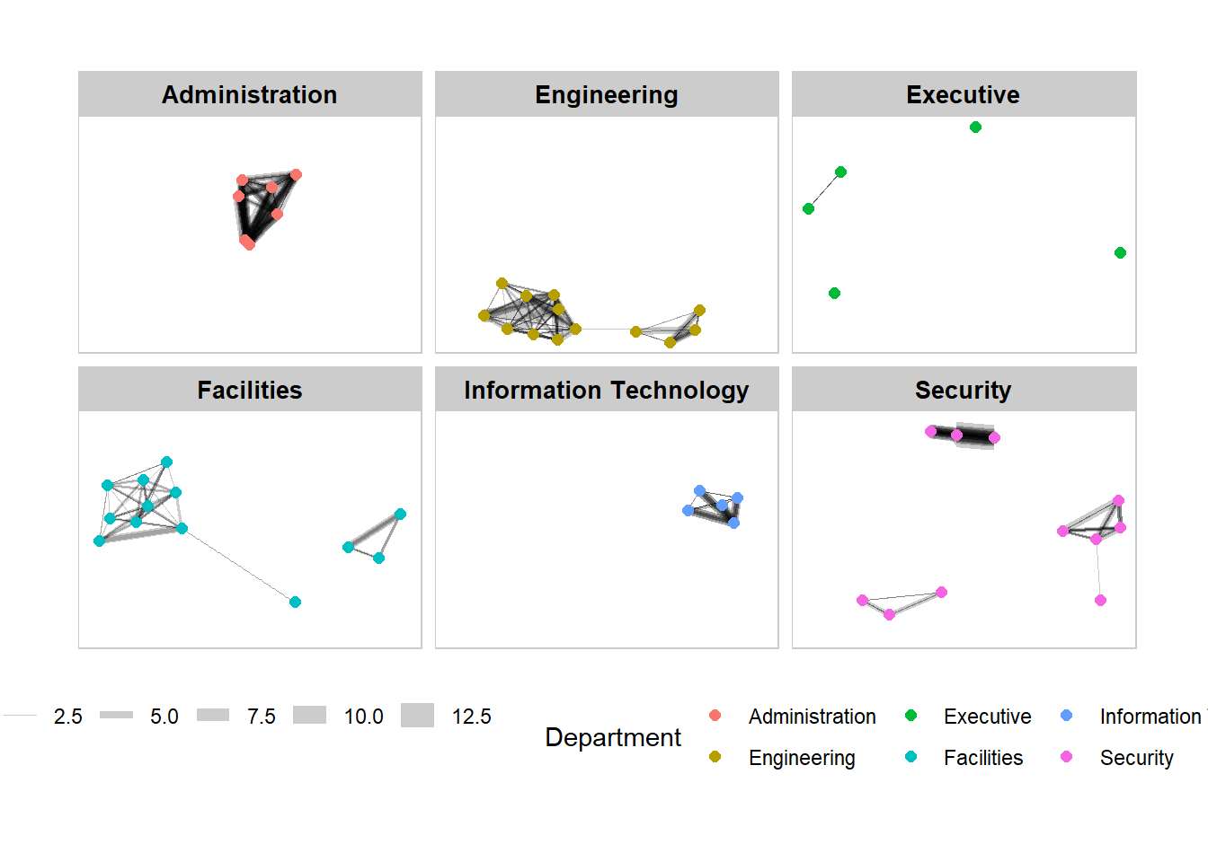
Network Metrics Analysis
Visualizing network metrics
g <- GAStech_graph %>%
  ggraph(layout = "fr") +
  geom_edge_link(aes(width=Weight),
                 alpha=0.2) +
  scale_edge_width(range = c(0.1, 5)) +
  geom_node_point(aes(colour = Department,
                      size = centrality_betweenness()))
g + theme_graph()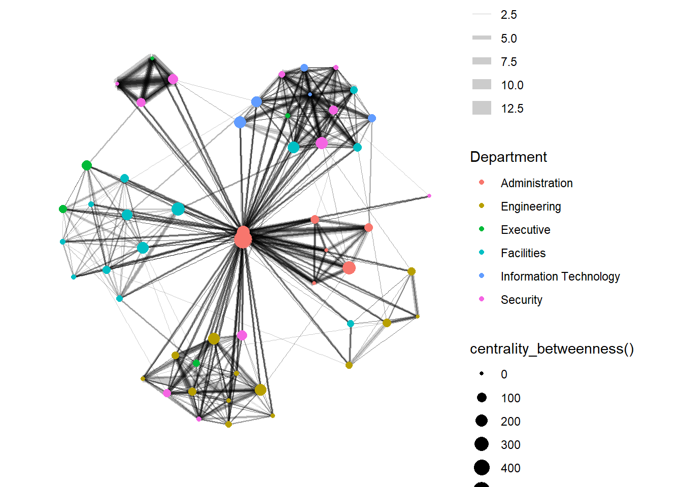
Visualizing communities
g <- GAStech_graph %>%
  mutate(community = as.factor(group_edge_betweenness(weights = Weight, directed = TRUE))) %>%
  ggraph(layout = "fr") +
  geom_edge_link(aes(width=Weight),
                 alpha=0.2) +
  scale_edge_width(range = c(0.1, 5)) +
  geom_node_point(aes(colour = community))

g + theme_graph()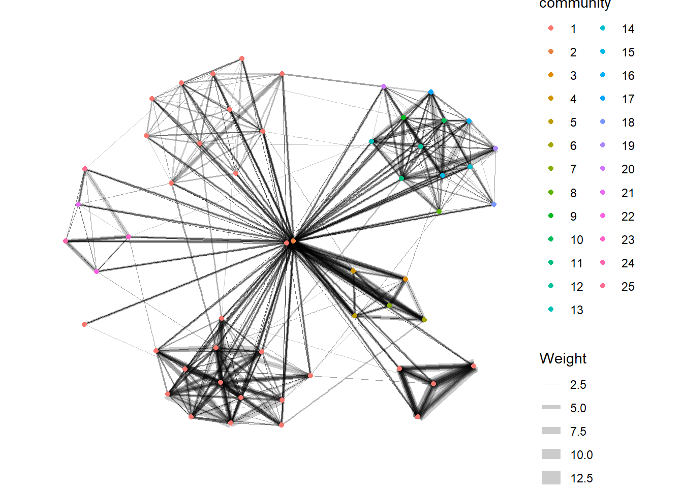
Plotting an interactive graph
GAStech_edges_aggregated <- GAStech_edges %>%
  left_join(GAStech_nodes, by = c("sourceLabel" = "label")) %>%
  rename(from = id) %>%
  left_join(GAStech_nodes, by = c("targetLabel" = "label")) %>%
  rename(to = id) %>%
  filter(MainSubject == "Work related") %>%
  group_by(from, to) %>%
    summarise(weight = n()) %>%
  filter(from!=to) %>%
  filter(weight > 1) %>%
ungroup()visNetwork(GAStech_nodes,
GAStech_edges_aggregated)Working with layout
visNetwork(GAStech_nodes,
GAStech_edges_aggregated) %>%
visIgraphLayout(layout = "layout_with_fr") Working with nodes
Rename group to department
GAStech_nodes <- GAStech_nodes %>%
rename(group = Department) visNetwork(GAStech_nodes,
GAStech_edges_aggregated) %>%
visIgraphLayout(layout = "layout_with_fr") %>%
visLegend() %>%
visLayout(randomSeed = 123)Working with edges
visNetwork(GAStech_nodes,
           GAStech_edges_aggregated) %>%
visIgraphLayout(layout = "layout_with_fr") %>%
visEdges(arrows = "to",
smooth = list(enabled = TRUE,
type = "curvedCW")) %>%
visLegend() %>%
visLayout(randomSeed = 123)Interactivity
visNetwork(GAStech_nodes,
           GAStech_edges_aggregated) %>%
  visIgraphLayout(layout = "layout_with_fr") %>%
  visOptions(highlightNearest = TRUE,
             nodesIdSelection = TRUE) %>%
  visLegend() %>%
  visLayout(randomSeed = 123)
Exploring Vast Challenge Data
Install and launching R packages
The code chunk below uses p_load() of pacman package to check if the relevant packages are installed in the computer. If they are, then they will be launched into R.
pacman::p_load(jsonlite, tidygraph, ggraph, visNetwork, tidyverse)Importing the data
MC1 <- fromJSON("data/MC1.json")Creating the graph
MC1_nodes <- as_tibble(MC1$nodes) %>%
  select(id, type, country)
MC1_edges <- as_tibble(MC1$links) %>%
select(source, target, type, weight, key)